A Brief Recap of Regression
In machine learning, when we want to make predictions about the value of some variable based on data, we can use regression. Training a regression model on data, we can make predictions about the value of the variable at a new location, even though we might be missing data at that location.
Example 1: Linear Regression
For a moment, let’s imagine we are a scientist observing some phenomena. We vary one parameter and observe our output. We could be developing a new medicine and looking at the relationship between dosage and efficacy. We could be developing a new metal alloy and looking at the relationship between the ratio of the components and the resulting strength. Regardless of our application, we will perform some experiments to get some data, which may look something like this:
[[Table 1]]
What can we do if someone asks us for the value of a point that we didn’t measure? We have many options thanks to machine learning. Let’s start with the most basic method: Linear Regression. In Linear Regression, we find the so-called ‘Line of Best Fit’, which is the line that minimizes the total error between itself and the data.
In our example, we get the following:
\[y=\beta_0+\beta_1x\]Example 2: Polynomial Regression
We can see both visually and from the MSE, that the line doesn’t quite represent the data very well. This means we likely don’t have the right model, so let’s beef up the linear regression into a second-order polynomial regression by adding a new term:
\[y=\beta_0+\beta_1x+\beta_2x^2\]We call this a ‘second order’ polynomial because it the highest power of \(x\) in the equation is two. Now that we have added the \(\beta_2x^2\) term, let’s see how well the model performs once we train it on the data.
This model performs much better, fitting the data pretty well with a lower MSE than linear regression, but it is not perfect. If adding a term improved the fit, then why don’t we try going to even higher orders?
We can see that as we increase the order, the fit gets better and better. For reasons we will not go into here, more is not always better, as the ugly monster named Overfitting can rear its head, but let’s ignore that for now.
The Gaussian Process
Now we understand what regression, we have to discuss the Gaussian Process. To do that, let’s review the Gaussian Distribution.
Example 3: The Uniform Distribution
To start, let’s imagine generating a random number. We could do this any number of ways, but for the sake of example, let’s use a 20-sided die to pick a number from 1 to 20. If we rolled this die many times, and counted the number of times each number appeared, we would find that all the numbers would show roughly the same number of times. This is called a Uniform Distribution, where all numbers are equally likely to appear.
\[x\sim U(1,20)\]Example 4: The Gaussian Distribution
Now, let’s roll 10 20-sided dice and average them out, repeating many times. What we will see looks quite different than the uniform distribution. Instead of any number being equally likely, we see a bell curve where 10.5 is the most likely result, with numbers just around 10.5 being the most likely, while numbers far from 10.5 are not very likely.
\[x\sim\mathcal N(\mu=10.5, \sigma=\frac{1}{3})\]This is the Gaussian Distribution. Gaussian Distributions are described by their mean value (the most likely value in the center of the distribution), and their variance (the spread of the distribution). In the above example, the mean of the distribution is 10.5 and the variance is about 3.33.
Example 5: The Gaussian Process
In our previous example, we implicitly assumed that all the faces on the dice were equally likely to appear, and that this would be true regardless of how many times you rolled them. Now, we will think about what might happen if the probability distribution representing a variable could change over time. We can imagine that there might be some functions that describe the mean and variance of a Gaussian distribution over some time, which could look something like this:
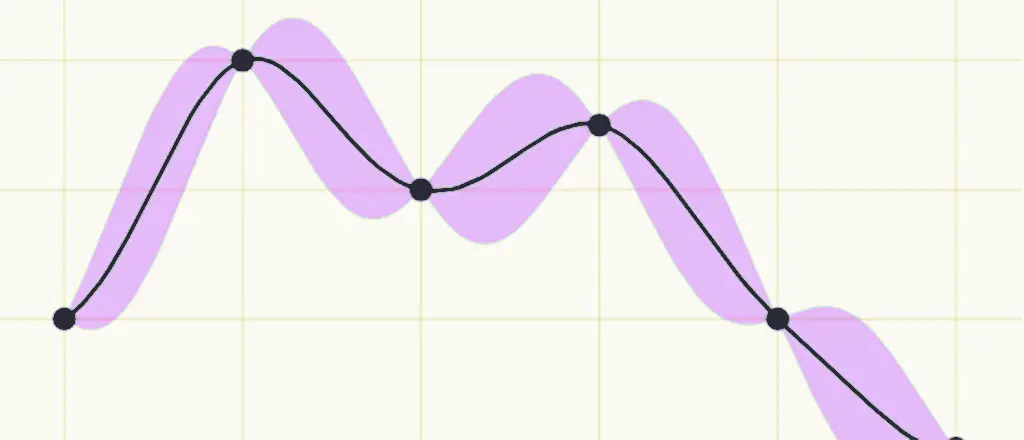
We can plot the mean value of the distribution over time on a chart and draw shaded regions around the mean to represent the variance. As the shaded area gets larger, that indicates that there is more variance at that point, and therefore more spread in the values.
This is the basis of a Gaussian Process. A Gaussian Process is a description of how the probability distribution of a random variable changes over time. Just as the Gaussian Distribution was controlled by its mean and variance value, a Gaussian Process is controlled by mean and variance functions.
Gaussian Process Regression
Now we can combine what we have learned about regression and Gaussian Processes into Gaussian Process Regression, which is the process of finding a Gaussian Process that best fits some data that we have observed. This means that we have to find the mean and variance functions for a Gaussian Process such that we minimize the error between our observed error and the model.
The most significant advantage that Gaussian Process Regression has over Polynomial Regression is that the variance at each point is directly accessible to us. Which means that when we are asked to make predictions at points we have not observed, we can not only report a predicted value, but also how confident we are in the accuracy of that prediction.
Thus, Gaussian Process Regression has become very popular for Machine Learning applications where uncertainty quantification is required, like financial forecasting. It also empowers other advanced machine learning techniques like Bayesian Neural Networks and Bayesian Optimization.
I hope this has helped to solidify your knowledge of this foundational topic in Machine Learning. Please reach out if you have any questions, comments, or corrections.